Energy minimization
In computational chemistry, energy minimization (also called energy optimization or geometry optimization) methods are used to compute the equilibrium configuration of molecules and solids.
Stable states of molecular systems correspond to global and local minima on their potential energy surface. Starting from a non-equilbrium molecular geometry, energy minimization employs the mathematical procedure of optimization to move atoms so as to reduce the net forces (the gradients of potential energy) on the atoms until they become negligible.
Like molecular dynamics and Monte-Carlo approaches, periodic boundary conditions have been allowed in energy minimization methods, to make small systems. A well established algorithm of energy minimization can be an efficient tool for molecular structure optimization.
Unlike molecular dynamics simulations, which are based on Newtonian dynamic laws and allow calculation of atomic trajectories with kinetic energy, molecular energy minimization does not include the effect of temperature, and hence the trajectories of atoms during the calculation do not really make any physical sense, i.e. we can only obtain a final state of system that corresponds to a local minimum of potential energy. From a physical point of view, this final state of the system corresponds to the configuration of atoms when the temperature of the system is approximately zero, e.g. as shown in Figure 1, if there is a cantilevered beam vibrating between positions 1 and 2 around an equilibrium position 0 with an initial kinetic motion, whether we start with the state 1, the state 2 or any other state between these two positions, the result of energy minimization for this system will always be the state 0.
Gradient-based algorithms are the most popular methods for energy minimization. The basic idea of gradient methods is to move atoms according to the total net forces acting on them. The force on an atom is calculated as the negative gradient of total potential energy of system, as follows:
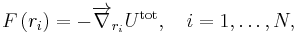
where ri is the position of atom i and Utot is the total potential energy of the system.
An analytical formula of the gradient of potential energy is preferentially required by the gradient methods. If not, one needs to calculate numerically the derivatives of the energy function. In this case, the Powell's direction set method or the downhill simplex method can generally be more efficient than the gradient methods.
Contents |
Simple gradient method
Here we have a single function of the potential energy to minimize with 3N independent variables, which are the 3 components of the coordinates of N atoms in our system. We calculate the net force on each atom F at each iteration step t, and we move the atoms in the direction of F with a multiple factor k. k can be smaller at the beginning of calculation if we begin with a very high potential energy. Note that similar strategy can be used in molecular dynamics for reducing the probability of divergence problems at the beginning of simulations.

We repeat this step in the above equation t = 1,2,... until F reaches to zero for every atom. The potential energy of system goes down in a long narrow valley of energy in this procedure.
Though it is also called “steepest descent”, the simple gradient algorithm is in fact very time-consuming if we compare it to the nonlinear conjugate gradient approach, it is therefore known as a not very good algorithm. However, its advantage is its numerical stability, i.e., the potential energy can never increase if we take a reasonable k. Thus, it can be combined with a conjugated gradient algorithm for solving the numerical divergence problem when two atoms are too close to each other.
Nonlinear conjugate gradient method
The conjugate gradient algorithm includes two basic steps: adding an orthogonal vector to the current direction of the search, and then move them in another direction nearly perpendicular to this vector. These two steps are also known as: step on the valley floor and then jump down. Figure 2 shows a highly simplified comparison between the conjugate and the simple gradient methods on a 1D energy curve.
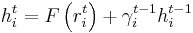
In this algorithm, we minimize the energy function by moving the atoms as follows,

where
and gamma is updated using the Fletcher-Reeves formula as:
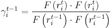
Here we note that gamma can also be calculated by using the Polak-Ribiere formula, however, it is less efficient than the Fletcher-Reeves one for certain energy functions. At the beginning of calculation (when t = 1), we can make the search direction vector 'h0 = 0.
This algorithm is very efficient. However, it is not quite stable with certain potential functions, i.e. it sometimes can step so far into a very strong repulsive energy range (e.g. when two atoms are too close to each other), where the gradient at this point is almost infinite. It can directly result a typical data-overrun error during the calculation. To resolve this problem, we can combine the conjugate gradient algorithm with the simple one. Figure 3 shows the schematics of the combined algorithm. We note for implementation that steps 2 and 5 can be combined into a single step.
Boundary conditions
The atoms in our system can have different degrees of freedom. For example, in case of a tube suspended over two supports, we need to fix certain number of atoms N* at the tube ends during the calculation. In this case, it is enough not to move these N* atoms in the step 4 or 8 in Figure 3, but we still calculate their interaction with other atoms in the steps 2 and 5. i.e. from mathematical point of view, we change the total number of variables in the energy function from 3N to 3N-3N*using the boundary condition, by which the values of these 3N* unknown variables are taken as known constants. Note that one can even fix atoms in only one or two directions in this way.
Moreover, one can equally adding other boundary conditions to the minimized energy function, such as adding external forces or external electric fields to the system. In these cases, the terms in potential energy function will be changed but the number of variables remains constant.
Here an example of the application of the energy minimization method in molecular modeling in nanoscience is shown in Figure 4.
Further information about the application of this method in nanoscience and Computational Codes programmed in Fortran for students is available in the following external links.
See also
- Graph cuts in computer vision – apparatus for solving computer vision problems that can be formulated in terms of energy minimization
- Energy principles in structural mechanics
External links
Additional references
- Payne et al., "Iterative minimization techniques for ab initio total-energy calculations: Molecular dynamics and conjugate gradients", Reviews of Modern Physics 64 (4), pp. 1045–1097. (1992) (abstract)
- Atich et al., "Conjugate gradient minimization of the energy functional: A new method for electronic structure calculation", Physical Review B 39 (8), pp. 4997–5004, (1989)
- Chadi, "Energy-minimization approach to the atomic geometry of semiconductor surfaces", Physical Review Letters 41 (15), pp. 1062–1065 (1978)